temp summaries to not cause conflicts in the repo (delete later)

3. Edge Detection

Edges seen as sharp brightness changes

Brightness changes and therefore edges are detected with threshold over the 1st derivative

Gradient approximation

in 2D, we calculate the gradient (vector of partial derivatives) that detects direction of the edge

• Magnitude = strength of edge
• Direction = towards brighter side We approximate the gradient by estimating derivatives with
• Differences (pixel difference)
• Kernels (same principle, using correlation kernels)

Noise workarounds

Noise causes false positives, so we smooth the image when detecting edges

Prewitt/Sobel ops make so we take into consideration the surrounding pixels to evaluate the edge Prewitt operator → take 8 surrounding pixels Sobel operator → likewise but central pixels weight 2x

Non-Maxima Suppression (NMS)

strategy of finding the local maxima in the derivative

• We need to find the gradient magnitude from the approximation
• We use Lerp from the discrete grid’s closest points To get rid of noise we apply a threshold

Canny’s Edge Detector

Standard criteria

1. Good detection → extract edges even in noisy images
2. Good localization → minimize found edge and true edge distance
3. One response to one edge → one single edge pixel detected at each true edge

Canny’s Pipeline

1. Gaussian smoothing
2. Gradient computation
3. Non-maxima suppression
4. Hysteresis thresholding → approach relying on a higher $(T_h)$ and a lower $(T_l)$threshold.

2nd derivative edge detection methods

Zero crossing = get point at 0 of 2nd derivative Laplacian operator (sum of second-order derivatives) to approx derivatives ${\nabla }^{2}I=\frac{{\partial }^{2}I}{\partial x^2}+\frac{{\partial }^{2}I}{\partial y^2}$

Laplacian of Gaussian (LOG)

Pipeline

1. Gaussian smoothing
2. Apply Laplacian
3. Find zero-crossings
4. Get actual edge from where the abs value of LOG is smaller

Parameter sigma controls smoothing degree and scale of features to detect (we blur more if edges are “bigger”)

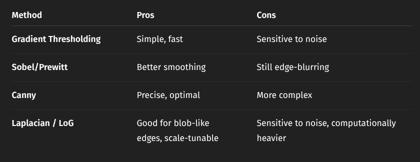
Comparison

4. Local Features

find Corresponding Points (Local invariant features) between 2+ images of a scene

Three-Stage pipeline

1. Detection of salient points
   • Repeatable, find same keypoints in different views
   • Saliency, find keypoints surrounded by informative patterns
   • Speed
2. Description of said points (what makes them unique)
   • Distinctive - Robustness Trade-off, capture invariant info, disregard noise and img specific changes (light changes)
   • Compactness, low memory and fast matching
   • Speed
3. Matching descriptors between images

Corner detectors

corners are the perfect keypoints as they have changes in all directions

Moravec Interest Point Detector → Look at patches in the image and compute cornerness (8 neighboring patches, look for high variation)

Harris Corner Detector

1. Compute image gradients (how intensity changes)
2. Build the structure tensor matrix $M$
3. Compute the corner response $C=\det (M)-k\cdot \text{trace}(M{)}^2$
4. Threshold & NMS to pick the best corners

Harris invariance properties

• Rotation invariance
• Partial illumination invariance (if contrast does not change)
• No scale invariance

Scale-Space, LoG, DoG

Key finding → apply a fixed-size detection tool on increasingly down-sampled and smoothed versions of the input image (trough Laplacian of Gaussian or Difference of Gaussian, its approximation) (LoG, DoG)

Scale-space → group of the same image at different computed smoothed scales $L(x,y,\sigma )=G(x,y,\sigma )\ast I(x,y)$ Where:

• G is the Gaussian kernel
• $\sigma$ controls the scale (blur amount)
• $\ast$ is convolution

Multi-Scale Feature Detection (Lindeberg) → makes us find which feature to extract at what scale

• Use scale-normalized derivatives to detect features at their “natural” scale.
• Normalize the filter responses (multiply by $\sigma$)
• Search for extrema (maxima or minima) in x, y, and $\sigma$ i.e., in 3D with LoG.

LoG → second order derivative that detects blobs (circular structures) $F(x,y,\sigma )={\sigma }^2\cdot {\nabla }^{2}L(x,y,\sigma )$ DoG → approximation of LoG $DoG=L(x,y,k\sigma )-L(x,y,\sigma )$ We build a pyramid of images blurred with different $\sigma$ and we compute the difference to find the extrema in 3D across (x,y, scale)

• We reject low contrast responses
• We prune keypoints on edges using the hessian matrix We get the optimal scale for each detail

DoG invariance

• Scale invariance
• Rotation invariance (compute canonical orientation so that we have a new reference system different from the image’s)

SIFT Descriptor

Scale Invariant Feature Transform → used to generate descriptors to match, outputs a feature vector based on grid subregions (takes small details from around the keypoint and remembers gradient orientation combinations)

Matching process

find closest corresponding point efficiently, classic Nearest Neighbour problem

• distance used is the euclidean distance
• ratio test of distances to eliminate 90% of false matches (distance to best match/second best), small ratio = confident match Indexing techniques are exploited for efficient NN-search
• k-d tree
• Best Bin First

5. Camera Calibration

We need to measure 3D info accurately from the 2D img Camera calibration → determining a camera’s internal and external parameters (focal length, distortion / position, orientation).

Perspective projection

3D point $M=[x,y,z{]}^T$ projected into 2D image point $m=[u,v{]}^T$ Function:

$$\{\begin{array}{l}u=\frac{f}{z}x\\ v=\frac{f}{z}y\end{array}$$

where: $f$ → focal length $z$ → depth (distance from the camera) This projection is non-linear, aka objects appear smaller with distance, all the rules of perspective

Projective Space

we need to handle points at infinity Projective space ($P^3$) → 4th coordinate for each point in 3D, $[x,y,z,w]$ $w\in [0,1]$, 0 means point is at infinity Express perspective projection linearly using matrix multiplication: $\tilde{m}=P\cdot \tilde{M}$

• $\tilde{M}$: 3D point in homogeneous coordinates $[x,y,z,1]$
• $\tilde{m}$: projected 2D image point $[u,v,1]$
• $P$: Perspective Projection Matrix (PPM) Canonical PPM (assuming $f=1$) $P=\left[\begin{array}{cccc}1& 0& 0& 0\\ 0& 1& 0& 0\\ 0& 0& 1& 0\end{array}\right]$

Image Digitization

continuous measurements into discrete pixel size, img origin Steps

1. Scale by pixel dimensions $\Delta u,\Delta v$
2. Shift the image center to pixel coordinates $(u_0,v_0)$ Intrinsic Parameter Matrix $A$ → captures internal characteristics of the camera $A=\left[\begin{array}{ccc}{f}_x& s& u_0\\ 0& f_y& v_0\\ 0& 0& 1\end{array}\right]$ Where:

• $f_x=f\cdot k_u$ →: focal length in horizontal pixels
• $f_y=f\cdot k_v$ → focal length in vertical pixels
• $s$ → skew (typically 0 for most modern cameras)
• $(u_0,v_0)$ → image center

CRF = Rotation matrix $\cdot$ WRF + Translation vector

Homography $H$

flat scene whose projection we can simplify to an homography $\tilde{m}=H\cdot \tilde{M}$ Where:

• $H$ → 3x3 matrix representing the homography
• $\tilde{M}$ → 2D coordinates in the plane + 1 in homogeneous coordinates (quadruple) Simplifies calibration, holds info about intrinsic parameters

Lens distortion

Barrel → outward bending Pincushion → inward bending we need to model non-linear functions to correct the image

What is calibration

Calibration estimates:

• Intrinsic parameters $A$ → Capture multiple images of a known pattern (e.g., chessboard)
• Extrinsic parameters $R,T$ → Find 2D-3D correspondences (image corner ↔ real-world corner)
• Lens distortion coefficients → projection equations

Zhang’s method

A Practical way to calibrate a real camera using images of a flat pattern

1. use a flat target (all $z=0$ )
2. form $m\leftrightarrow M$ pairs, get homographies $H_i$
3. Each homography relates image coordinates to pattern coordinates 4.5 points per image needed to compute $H_i$

Summary

Concept	What It Represents
$A$	Intrinsic matrix (focal lengths, image center, skew)
$R,T$	Camera pose (extrinsics)
Homography $H$	2D projective mapping for planar scenes
Distortion	Lens imperfections modeled with parameters
Zhang’s Method	Practical way to calibrate a real camera using images of a flat pattern

Part 2

---

6. CNN recap (Convolutional Neural Networks) TODO