Notes taken by Luizo ( @LuigiBrosNin on Telegram)
- Exam info
collapsed:: true
- Presentation like in the thesis of a paper in the drive “StudentCBD” folder
- Free choice, no overlap in here (you need to compile the form to get in) (links for 2024/25)
- CHANGE THE REFERENCES FROM THE TEMPLATE PLS
- You’ll get the slides in google slides through mail after compiling the form
- Presentation in 30m time
- “expand the scopes of the paper”
Theory
Appunti Francesco Corigliano i studied here anyway (Italian notes)
- 1 Intro Models
- 2 Intro XML
- 2.2 SQL/XML - Relational Data and XML
- 2.3 XQuery - XQuery language
- 2.4 XQuery in DBMS - XQuery on DB2, Oracle and SQL Server
- 2.5 NoSQL
- 3.1 IR - Information Retrieval
- 3.2 Ranking
- 3.3 Web Information Retrieval
- 3.4 IR Evaluation
- 3.5 IR Advanced methods
- 4.1 Data analytics
- 4.2 Data Warehouse
- 4.3 Data Mining
1 Intro Models
Relational → structured (basically)
NON RELATIONAL MODELS
-
boolean model not usable, searches are not 100% relevant.
-
no scheme
Queries can’t manipulate data, but can retrieve them ordered by relevance
RELATIONAL MODELS
-
set-based
-
not nested, not ordered
-
distinction between schema and data
-
boolean model
-
XML can represent it
SEMI-RELATIONAL MODELS
-
shows proprieties of both structural and non-structural data
-
retrospective-built schema, always evolving
-
list-based
-
XML is the primary format
-
many query can’t be written in SQL without compromises (recursion, slowness)
2 Intro XML
eXtensible Markup Language, comes from SGML (Standard Generalized Markup Language)
both can be used to define markup languages for many domains
XML Structure:
- Prolog → info for doc interpretation (eg. xml version, document type definition DTD)
- Document Body →an element that can contain more nested elements and comments
-
each element is enclosed in a
<tag></tag>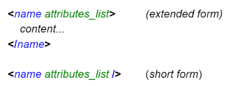
-
names are case sensitive
-
values of attributes must be contained in
‘’or“” -
attributes can’t have the same attribute more than once
-
data must be within the enclosed tag
-
2.2 SQL/XML - Relational Data and XML
collapsed:: true
XML is used to exchange data between apps and represent structured data.
SQL/XML is a bridge for archiving locally these data in a relational manner
2 main functions to achieve conversions
-
XML Extraction (SQL → XML, easy) - Mapping each data type that can be represented in the XML in a table (name of table → name of doc, every line is a row element and each value (column) is included in an element with the attribute name) - Extracting data using XQuery: SQL → XML (SQL/XML) 2. XML Archiving (XML → SQL, complex) - Columns are Object-Relational, to archive XML fragments in a single field - Fragmenting documents to be stored piece by piece
SQL/XML Language → SQL extension that contains constructors, routines, functions to support manipulation and archiving of XML in a SQL db.
- Operators
-
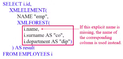
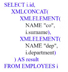
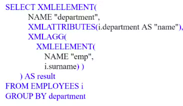
XMLELEMENT → creates an XML element with args
- Name → given explicitly trough a constant
- Content → you can specify any objects, elements or strings ( concat op → || )
- attributes → optional list
-
XMLATTRIBUTES → params corresponding to attributes, default name as the attr name
-
XMLFOREST → produces a list of simple elements, same params as XMLATRIBUTES
-
XMLCONCAT → concats a forest of elements
-
XMLAGG → groups tuples based on one or more attributes, with GROUP BY op
-
XMLGEN → specify the XML code to insert, you can use variables between
{}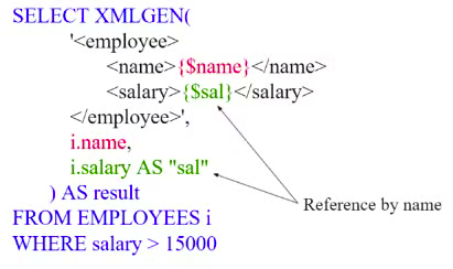
The result gets calculated considering the SQL, making a SELECT * and then building the requested attributes 1 by 1.
-
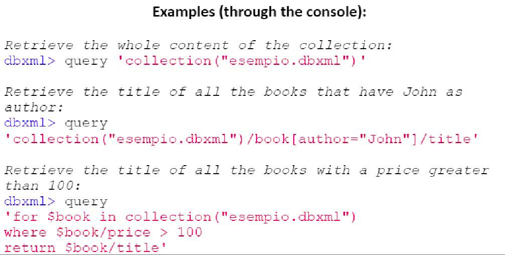
2.3 XQuery - XQuery language
XQuery can be used to access XML expressed data and has XSLT functions (eXtensible Stylesheet Language Transformations).
XQuery operates on sequences, that can be atom values (eg. “hello” string, “3” integer) or nodes.
an XQuery expression can receive in input or sequences, and output an ordered and not-nested sequence.
-
Ordered →
-
Not-nested →
-
sequence = element → collapsed:: true
Operators:
,,to,union (same as | ),intersect,except- Equivalents →
- union
- intersect
- except
Nodes
Attributes: when XQuery extracts attributes, they’re not ordered, but they get inserted in a sequence, preserving the order.
Text: the value of the string of each node of type document / element is the ordered concat of all text childs.
two text nodes can’t be adjacent (eg.
Jane Doe → “Jane Doe” is the text node, “Jane” + “Doe” are not 2 different text nodes)Nodes can be of text, integers, date type.
Path Expressions
Used to extract values and proprieties from nodes and trees.
"doc_name.xml"/child:doc/child:chapter/child:selection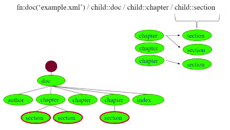 Each path gets evaluated in a context (a sequence of nodes with extra info, such as position) and produces a sequence.
It then gets evaluated, and the context used is the sequence in the previous step, and so on.
Stair step structure → expression to path, 3 step procedure:
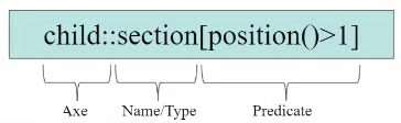
- Axe → select the nodes relative to the position of the context node
-
self::
-
child::
-
parent::
-
ancestor::
-
descendant::
-
following-sibling:
-
preceding-sibling::
-
attribute::
-
descendant-or-self::
-
ancestor-or-self:: 2. Test → filter result nodes based on:
-
Name
- child::section → return only the section tag within the children
- child::* → return all children
- attribute::xml:lang → returns xml:lang attribute
-
Type
- descendant::node() → returns all descendant nodes.
- descendant::text() → returns all descendant text nodes.
- descendant::element() → returns all nodes of descendant elements.
-
Both → descendant::element(person, xs:decimal) → returns person elements of type decimal 3. Predictate → filters nodes on generic criteria, each step can terminate with one or more predicate, inb
[]to filter even more, like an array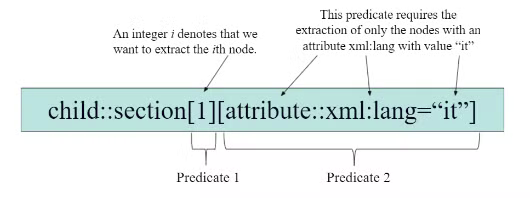
predictate is true if -
expression returns a single integer value
-
the position of the subject node corresponds to a integer value (
child::chapter[2]returns the 2nd child of the chapter tag) -
1st element is a node
-
child::chapter[child::title]→ returns all chapter tags who have a title tag child. -
child::chapter[attribute::xml:lang = "it"]→ return all chapters with the lang attribute set to “it”.predictate is false if the expression returns a non-empty sequence.
Complete path expressions → starts with
/or//to contain the root of the document or all the nodes respectively.Shortened syntax
-
-
Omission of Child → child::section/child::paragraph = section/paragraph
-
Substitution of Axe with @ → para[attribute::type=“warning”] → para[@type=“warning”]
-
Substitution of descendant-or-self::node() with
**//**→ div/descendant-or-self::node()/child::paragraph → div//paragraph -
Substitution of self::node() with
.→ self::node()/descendant-or-self::node()/child::para → .//para -
Substitution of parent::node() with
**..**→ parent:node()/child::section → ../sectionFLWOR Expressions
For, Let, Where, Order by, XQuery equivalent of SELECT-FROM-WHERE, but defined by binding variables
- Return, creates the result
-
For and Let create a list of tuples (all possible associations) 2. For → associates one or more variable to the expressions
iterates all elements in a variable (like )
- Let → declares a variable basically
you can aggregate expressions to functions: grouping elements to evaluate them to find numbers (min, max if they’re numbers)
- Where → filters a list based on a condition (basically an if in a for)
- Order by → orders the list based on parameters
- Comments →
(: like this :)
-
Join example
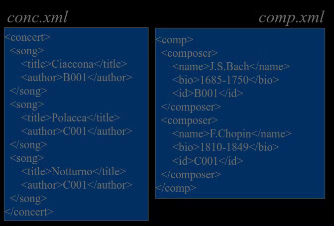
tablesWe want to produce a screening schedule listing songs, author and birth + death dates.
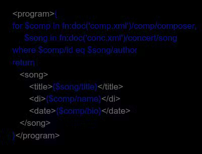
query
outputConditional expressions
basically if-then-else, in xQuery constructed like this
if ($product1/price < $product2/price)
then $product2
else $product1
Comparison operators → =, !=, <, ⇐, >, ≥
they act on sequences, meaning
$book1/author = “Luizo”is true if at least 1 selected node “author” is equal to Luizo.These operations are not transitive:
(1, 2) = (2, 3) = TRUE
(1, 2) != (2, 3) = TRUE
XPath 2.0 adds → eq, ne, It, le, gt, ge
Expressions with quantifiers → XQuery variables are often associated with sets of objects instead of single values (eg.
for $lib in doc books.xml/books/bookassigns<book>elements)specific operators can verify proprieties of objects eg:
some$emp in //employee→ equivalentevery$imp in //employee→ equivalentStandard functions
input functions, necessary to obtain the XML code to make the query
-
fn:doc('bib.xml')→ access a document -
fn:collection('compositors')→ access a set of documentsNode sequence functions
-
fn:position()→ current node position -
fn:last()→ of nodes -
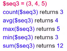
fn:count($elements)→ node sequence cardinalityAggregated functions
2.4 XQuery in DBMS - XQuery on DB2, Oracle and SQL Server
DB2
DB2 can insert XML type columns into relational tables trough the INSERT + XMLPARSE function.
XQuery queries are inserted trough the SELECT clause trough XMLQUERY, which returns XML fragments
XMLEXISTS → in the WHERE clause
XMLTABLE → in the FROM clause
DB2 supports all axe path expressions, all nodes and all tests for the XPath standard.
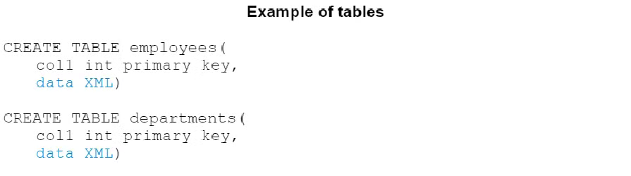
to create a XML table, specify XML as data type in a column.
-
DB2 Examples of XMLPARSE | XMLQUERY (literally just an XPath tutorial lol)

to insert XML data, we can use XMLPARSE, we can choose to maintain the white space.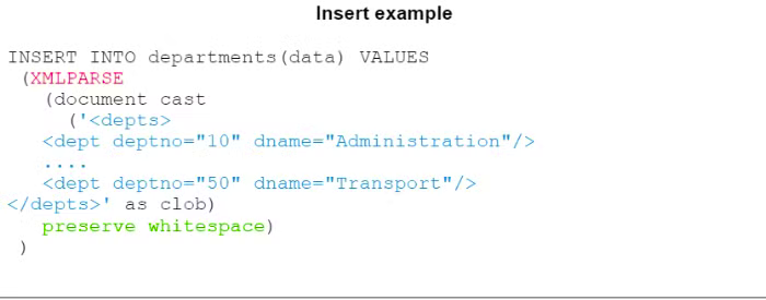
SELECT example that extracts departments and puts them in<deptName>trough XMLQUERY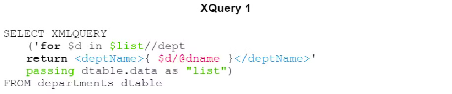
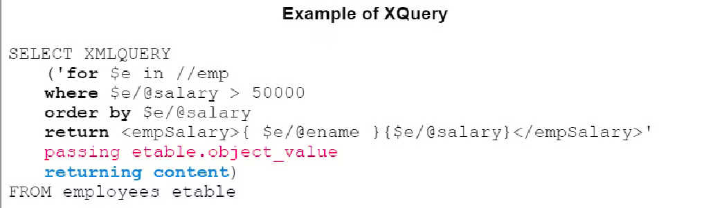
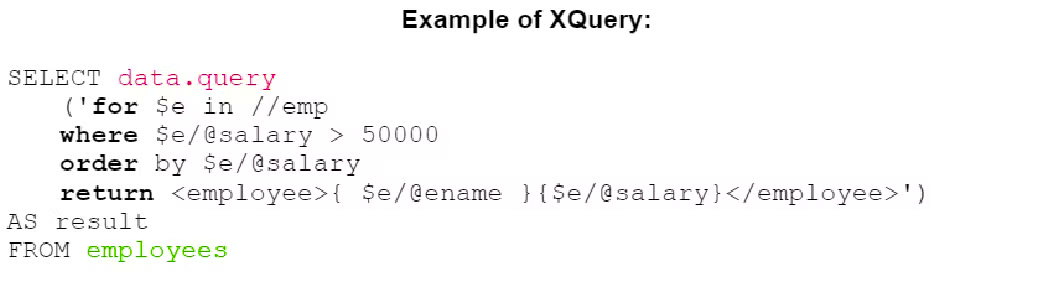
passing → specifies the XML fragment we’re working on, in the example what gets passed is the content of the departments as a list, so it creates a$listvariable that we can use inside the query.example that extracts names and salaries of all employers who gain > 50k and inserted in
<empSalary>and ordered by salary.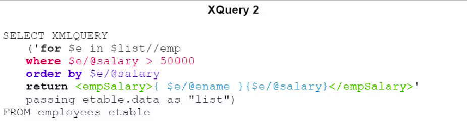
example that uses ==letandavg== to see the average salary of the department in which each employee works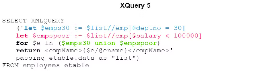
Union operator example (basically an AND)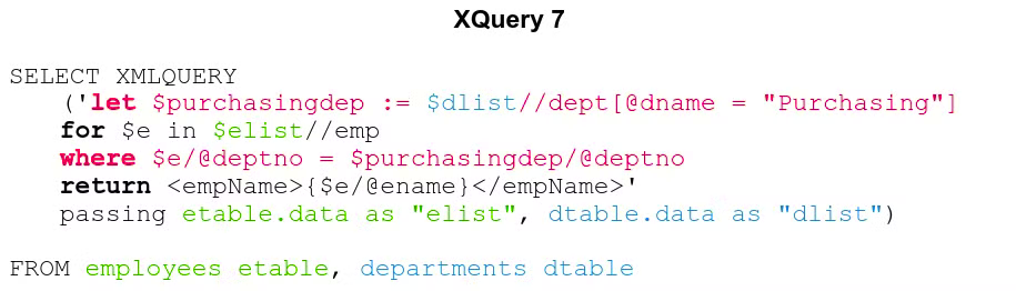
Join equivalent example. We’re passing both employees content and departments content for it to work.
Join + let example to get for each department, name + sum of salaries from that department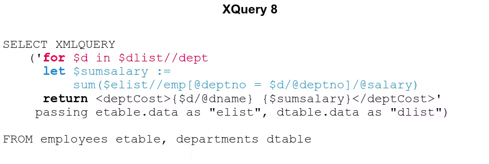
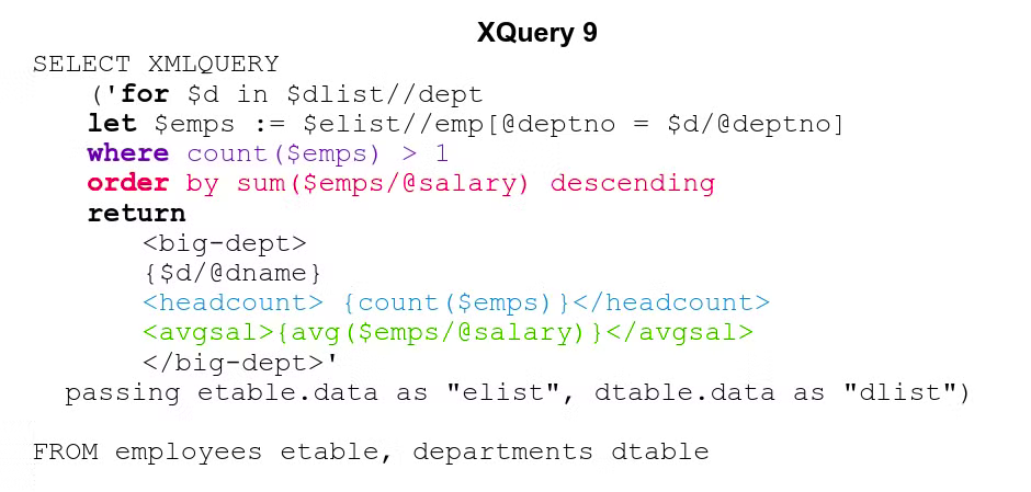
Mishmash of all previous examples:for each department, we want the number of employees (BLUE), the average salary (GREEN). results must be sorted by the sum of the salaries (RED) of each department, and filter out departments with only 1 or less employees (PURPLE)
XQuery in oracle DB
non-supported functions:
-
version encoding
-
xml:id
-
xs:duration (use xs:YearMonthDuration or xs:DayTimeDuration)
-
schema validation feature
-
module feature
-
no standard functions for regex
-
fn;id, fn:idref are not supported
-
fn:collection with no arguments not supported
Table creation → with XMLType keyword
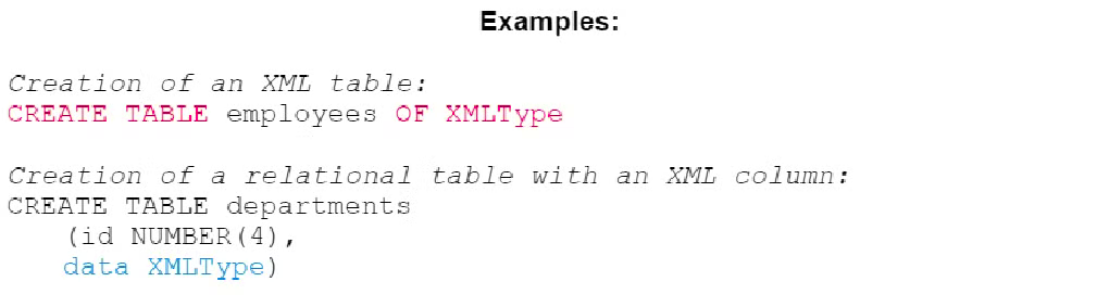 XMLType can be implemented as
- LOB (Large OBject) → string
- Structured Storage → automatic tables that follow the XML schema, preserving the DOM
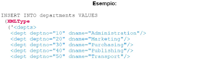
inserting a XML fragment in a table → XMLType into an insert followed by the string in XML
-
-
Oracle Examples
XQuery example in Oracle, same example as DB2
Join equivalent example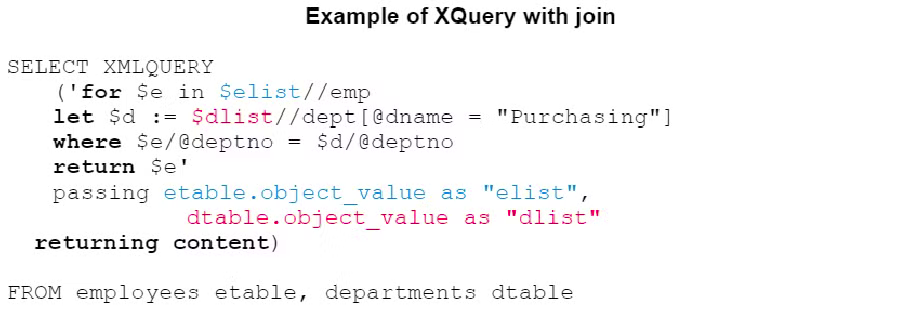
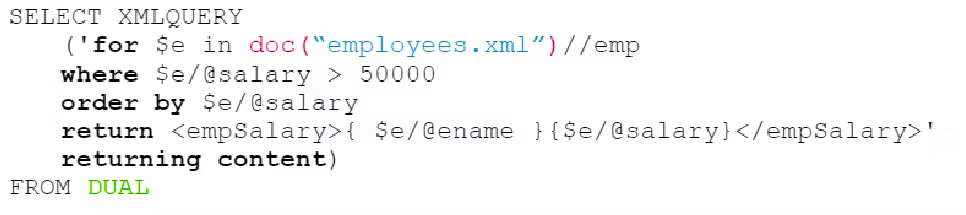
we can usedoc()to query XML files directly without inserting data in tablesa DUAL empty table is present in all default Oracle database, used as a foobar option since “FROM” is required in SQL
XQuery on SQL Server 2012
non-supported features:
-
Sequences
- must be homogeneous (composed of nodes or atomic values)
- to construct is no supported
- union, intersect, except cannot be used to combine node sequences
-
Path Expressions, they are only supported:
- child, descendant, parent, attribute, self, descendant-or-self Axes
- comment(), node(), processing-instruction(), text() Types
-
FLWOR
- LET will be inserted every mention of the variable, meaning it will be recomputed each time the variable gets referenced
-
idiv and not are not supported
SQL Server
Table creation → with XMLType keyword
 to insert data in the table, INSERT op with a XML fragment under a string
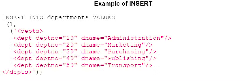
-
Query example in Oracle Berkeley DB XML
same query as before, but without “passing”Oracle Berkeley → set of libraries that can be used inside common programming languages to manage an XML DB
Major Operations
Create a container
- document-based container → document archived as delivered to the system
- node-based container → document gets turned into nodes and archived separately, they can be modified afterwards
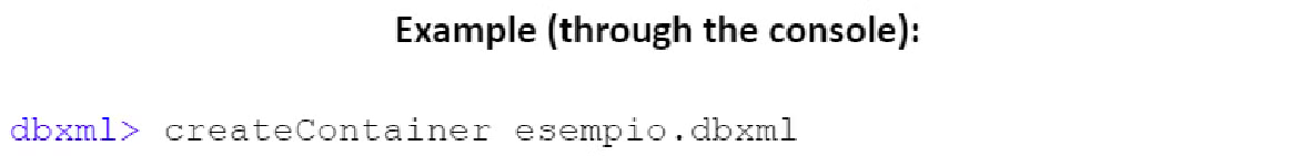 containers are comparable to table in relational DBMS
we can use “
putDocument <namePrefix> <string> [f|s|q]” to insert documents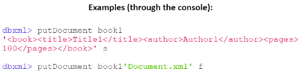 parameters
f → string is a path to an XML
s → string is a XML fragment
it’s possible to bind a schema of a XML document to a table so that you can only insert documents that satisfy that schema into the database
Indexes can be created which improve performance
retrieving documents in a container can be done trough XQuery queries
2.5 NoSQL
means a non relational database, there are 225+ systems that are NoSQL
Proprieties of BASE (ACID equivalent)
-
no ACID proprieties
- weak consistency
- more powerful
- easy to use and fast
- optimist
-
no Schemas → replaced by non relational model, key-value, doc, graph
-
Availability → always data availability, but “failure” or inconsistent data are also possible result
-
Soft state → the state of the system can change overtime
-
Final consistency → sooner or later data will be coherent, but no consistency verification on every transaction
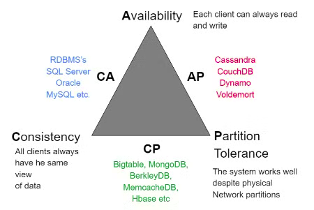
CAP compromise (triangle)
- Consistency → works or not
- Availability → every request gets an answer
- Partition Tolerance → still works on data loss, a single node error doesn’t cause a system collapse
 in NoSQL, there is no schema, no unused cells and data types are implicit. most considerations are executed at application level.
 -
Aggregation → elements are gathered in an aggregate (document)
-
Aggregate → cluster of domain objects that can be treated as an unity. aggregates are the base example of transaction and archiving of data
-
Polygot persistence → Hybrid approach at data persistence, there are many db models made to solve different needs.
Schema replacements
Key - Value → hash table
Key → string
Value → any data type, usually a block of data not interpreted (binary / json), memorized as blob.
4 base operations
- Insert(key, value)
- Fetch(key)
- Update(key)
- Delete(key)
Data model of documents → XML, JSON, text or binary BLOB
any tree structure can be represented as XML or JSON, similar to key-value, but the value is a document.
pros:
-
Rich data structure → incorporates data in secondary documents and arrays, supports advanced queries and indexing
-
aggregated data in a single structure → good performance
-
dynamic scheme → data can quickly adapt to necessities
Columnar data model → archiving tables as columns of data instead of rows
Columnar → extensions to traditional tables (adding info)
Graph data model → graph algorithms are used, graph theory is used to structure data
-
vertical scaling
-
transaction
-
ACID
3.1 IR - Information Retrieval
Means finding non structured material that satisfies an information need, usually about web search, social media, local laptop usage.
Document → web page, email, book, article, messages, word, pwp, pdf, forum posts, etc
Common proprieties → meaningful text content + non structured data
Collection → series of documents (static collection)
Query → set of key words to express an informatory need
Our objective → recover relevant docs and help the user complete the activity
IR vs Data Retrieval
Data retrieval (DBMS) → database record
-
structured into fields
-
consistent values and types
-
pre-defined formats for storage
IR → text document
-
unstructured
-
can contain any kind of data
-
expressed in natural language
Query language
-
based on a formal grammar
-
answer is independent from implementation
-
answer → predictable set of records that are true under a query
Search language
-
based on keywords
-
can be interpreted differently
-
answer → ranked list of results based on likeliness from query
Text comparison
compare the query text with the document text and determine coherence is the main problem in IR.
We need a pertinence-based ranking instead of an exact match, to accomodate the natural language.
Retrieval models
- classic models → boolean retrieval, spatial-vectorial
Boolean retrieval → simple, sees documents as bag of words, precise
Incidence vectors → slightly complex queires would require a matrix dimensions of billions, to save space we save the 1 positions.
Inverted index → we use posting-lists to avoid wasting memory with fixed arrays
- probabilistic models → BM25, linguistic models
- combining evidence → inference networks, learning to rank
Text processing
-
Tokenization → cut character sequence into word tokens
-
Normalization → map text terms to same “normal” form (eg. U.S.A and USA)
-
Lemmatization → reduce to simple correct forms (eg. the boy’s car are different colours → the boy car be different colours)
-
Stemming → different forms of a root to match (authorize, authorization)
-
Stop words → omit very common words (the, a, to, of)
-
Dictionary → lexical indexes, used for autocorrection too
3.2 Ranking
Ranking recovery → the system returns a ranking “on top” while going for a query
Vector Space Model (VSM)
Ranking mode, documents are represented by vectors or matrix based on weight of words
 Docs as vecs proprieties
-
|Vectorial space as |V|-dimensional|
-
terms are axes of space
-
documents are points
-
millions of dimensions on search engines, most empty
Query as vecs proprieties
-
represents queries as vectors in space
-
classifies documents based on distance (near → vectors are alike)
-
classifies documents on relevance, from least distant
Term Frequencies (TF) → assigning a weight for each term in a vector space, based on frequency.
→ term frequency of term in document
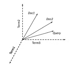
Vector space distance
 D1,D2,D3 are phrases, Q is a query
Euclidean distance → straight line distance between the final points, doesn’t work with what we need to do
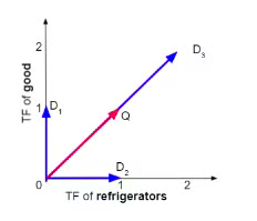
Using angles
by taking the angle most similar to the vector phrase, we achieve what we need
classifying documents by descending angles and ascending cosine are the same, so we use that
Cosine is a monotone descending function (0 to 180), meaning it is inversely proportional of the angle
Cosine similarity
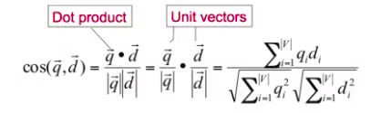 → tf weight of query term
 → tf weight of document term
is the cosine similarity between the 2 angles, or the cosine of the angle between and .
Search engines
knowing what the user wants
-
information need → localizing info that we’re looking for
-
user query → the terms that express the information needs
-
query intent → the user activity
how to search trough millions of documents
-
Topological network measures (PageRank)
-
field boosting measures (Title, subtitle, body on different weights)
-
semantics and time space proprieties (freshness of page)
Search Engine Results Page (SERP)
users click on the better results, 1st result is clicked 10x as more as the 6th one
to be in the 1st position, the cost per click is 10 times higher than the 6th one
common words are less informative than less common terms
Document Frequency → number of documents that contain
Inverse Document Frequency → how rare is a word
-
→ number of docs
-
we apply the logarithm to mitigate the exponential growth of really common words (Zipf law)
TF IDF get used a lot together for better estimates
Probabilistic Models
using probability to estimate relevance is the most efficient way of retrieving docs
- Okapi BM25 (weighting scheme) → uses doc length, term frequency and rarity to ponder documents
- similarity score is between 0 and 1
- params
- k1 → saturation and term frequency, default is 1.2
- b → controls how much weight the vector norm of the doc length has, default is 0.75/ (0 → no normalization, 1 → complete normalization)
- Language model → assigns a probability on a word sequence trough probability distribution
- each language model is tied at each doc of the collection, classification is Q query under the model
- Unigram LM → text generation is to extact words from a bucket following probabilty
- N-grams LM → same, but uses N previous words to calculate the next one
Raking efficiency
ranking is computationally costly, even more if the query is complex
some efficiency checks:
-
how we access document is relevant
-
we’re mostly not interested in lesser relevant documents
we have a latency limit to satisfy the user, and we can’t assign a complete score to each document for each query
TAAT vs DAAT
TAAT (Term At A Time) → scores for all docs concurrently, one query term at a time
DAAT (Document At A Time) → total score for each doc
Secure ranking → guarantees K results as the highest scored overall
Non-secure ranking → docs near K could be enough
-
index elimination → consider only rare terms (high IDF), consider only documents that contain a lot of query terms
-
champion lists → pre-compute scores of top relevant documents
3.3 Web Information Retrieval
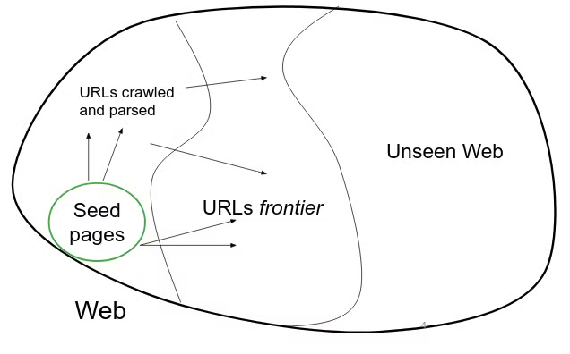
Web crawling → process of gathering pages from the web
Crawler (spider)
takes known seed URLs, fetches and parses them and puts them on a queue called URL frontier, then fetches each URL on the frontier and repeats
 a crawler requires
Robustness → web scan on distributed machines
-
malicious pages (spam - spider traps (endless pages))
-
latency, webmaster conditions, depth of hierarchy scan, mirror sites and dupe pages
Politeness → sever web policies
explicit → specs from webmasters on which portions can be crawled
implicit → avoid hitting same site too often
robots.txt →explicit protocol, gives limited access to a website, defines rules
URL Frontier
can search trough breadth first (only 1st page of site) or deep first (stops at 1st page without other links)
rankings are constructed combining
-
content → can use RI models like probability based ones
-
popularity → calculated trough hypertext links analysis using one or more link analysis models
Simple link analysis → good nodes do not go into bad ones, so we mark them as good
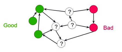 Citation analysis → popularity estimate
 -
co-citation of articles means they’re correlated
-
indexing of citation for author searches
-
Page-Rank preview
Page-Rank → 0 to 1 assignment to each node from the link structure. for each query, this gets integrated into the search engine results to define the classification list.
the probability of a user being on a given site (during browsing) is that site’s page-rank.
some factors Google uses for raking:
-
Page ranking
-
language (phrases, errors, synonyms)
-
time characteristics (some queries look for recent indexing, like news)
-
personalization (history, social ambient, etc)
HITS → Hyperlink-Induced Topic Search
useful for wide argument queries, 2 series of correlated pages
-
Hub page → points to many trusted pages
-
Authority page → pointed by good hub pages
Semantic search → graph search over structured knowledge rather than text speech
3.4 IR Evaluation
measuring relevance
- benchmark doc collection
- benchmark suite of queries
- human assessment of relevancy
user needs are translated into a query, but relevancy is assessed by the user.
Relevance judgments
-
Binary (relevant \ not relevant)
-
considering all sets of docs is expensive
-
depth-k pooling solution → take the top- docs of different information retrieval systems, having a pool instead of the entire collection
Collections Text REtrieval Conference (TREC) → biggest available web collection, 25m pages.
Mechanical Turk → presenting query-doc pairs to low-cost labor on online crowd-sourcing platforms, a lot of variance in resulting judgements
the effectiveness of an IR system is dictated by
-
Precision → relevant results / total results
-
Recall → relevant results / relevant docs in the collection
@K → parameter, threshold rank, made to ignore documents < K
Average Precision → the average of @K precision calculated on Ks were it was retrieved the relevant result, stops at Recall@K = 1
Mean Average Precision (MAP) → macro-average, aka measured from the average on all queries
Precision 0 → if a relevant doc never gets retrieved
non-binary notion of relevance → spectrum of relevancy, measure is DCG (Discounted Cumulative Gain) or NDCG (Normalized Discounted Cumulative Gain)
3.5 IR Advanced methods
Synonymy → using different words to refer to the same thing, it’s a problem that impacts the majority of IR tools’ recall.
Query extension → expanding the query with synonyms
eg. “car” → “car automobile vehicle automobiles”
there are many query extension techniques
Correlated terms
-
trough wordnets
-
co-occurring terms in the same documents or in an adjacent relevant document
Thesaurus query expansion → automatic expansion based on vocabulary is not effective (a word means different things in different contexts)
we can use co-occurencies based on:
- Dice’s coefficient → , higher the score, the more correlated the words. in practice, we have:
where:
→ words
→ documents containing a and b respectively
→ documents containing both
- Mutual information → based on probability:
where:
→ words
→ probability of the word existing in a window of text
→ probability of the words together existing in a window of text
This method inherently favors terms of low frequency
- Expected mutual information → fixes the problem with low frequency with P(a,b):
- Pearson’s Chi-squared () → confronts the number of co-occurencies with the expected number of co-occurencies if the words were independent and normalizes it (dividing it) with the expected number
measures are based on documents or smaller parts.
Query expansion with relevance feedback (RF) → makes use of refinement techniques based on user feedback
Pseudo RF (blind relevance feedback) → automates the manual RF, calculating it based on the first results
Machine learning (ML) and IR → building a classifier using AI, based on term frequency in body and title, doc length and doc popularity (pagerank).
our goal is to build a classifier for relevant and non-relevant docs.
“luckily”, lots of training data is available.
4.1 Data analytics
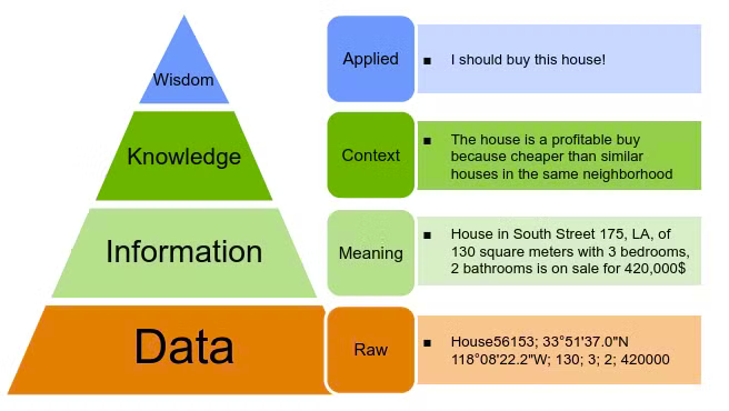
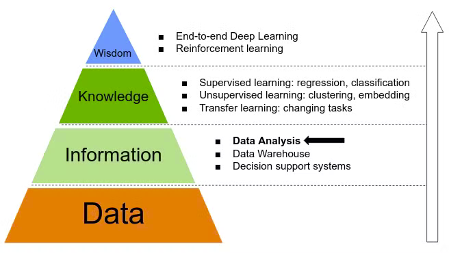
DIKW Pyramid → how information is defined along with knowledge and wisdom
 Data analysis → extract information from the data
 we can extract information as
-
summaries, as the average of a group of numbers
-
association, creating relations
Population → set of relevant objects to get info from
es. all Los Angeles houses, all university students, all recipes of grocery stores
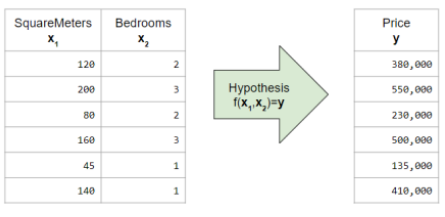
Record → tuple of values, characterizes a population element (es. a house’s square meters, price, etc)
Variable → name of the value of a record
-
Numerical variable, we can apply arithmetics. the numbers can be discrete or continued.
-
Categorical variable
-
Ordinal, if they can be ordered (eg. school grades)
-
Nominal, eg. colors
Dataset → a set of records becomes a unique table
Descriptive statistic → indicators that can identify the statistical proprieties of a population based on a single variable
Centrality
Arithmetic mean → used to fill missing data, sensible to anomalies
we can maintain the same mean by replacing missing data with the mean result.
Median → effective value of the observations, immune to anomalies, but needs ordered data.
Mode → most frequent effective value, robust to anomalies, can be applied to categorical variables.
Variation
Squared Deviation → measures each difference between any and the average observation →
deviation is higher the more values are far from the average, and the more values, the higher the deviation.
Variance → (written as or ) normalizes the Squared deviation by the number of values: Single variable indicators
-
-
Min → minimum value in observations
-
Max → maximum value in observations
-
Range → difference between max and min Multiple variable indicators in descriptive statistic, they describe the relation between variables, aka how and if they’re linked (eg. houses price to squared meters).
-
Covariance
-
Correlation Association measures
-
Covariance → strength of relation between 2 variables if the covariance is high (many and diverge at the same time) there’s a relation Positive covariance → directly proportional, X and Y diverge in the same direction Negative covariance → inversely proportional, X and Y diverge in opposite directions Variance is subject to change value based on measurement units, big values give big results, which is not a problem in correlation
-
Correlation → divides covariance by the product of the standard deviations, limiting values between -1 and 1.
- tends to -1 → opposite variation, inversely proportional
- tends to 1 → same variation, directly proportional
- tends to 0 → independent variation, linear relation
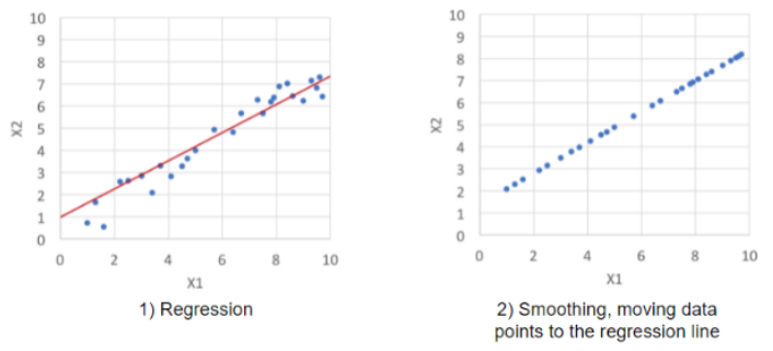
Dispersion and regression graph
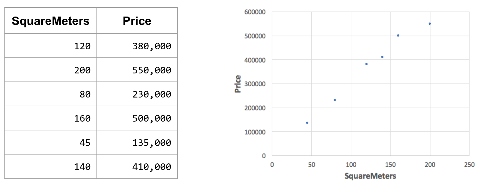 Useful to visualize the values, see if there’s an association
4.2 Data Warehouse
Data Warehouses → operative database, supports software apps and has big repos that consolidate data from different sources.
-
Is updated offline
-
Follows the multidimensional data model
-
Needs complex queries to analyse and export data (computationally costly)
-
Implemented using the star or snowflake scheme to efficiently support OLAP queries.
Decision process based on data Companies may use data to take informed decisions Decision makers need to know the techniques of the data models
-
Data Warehouse proprieties:
-
Oriented at subject → targets one or several subjects of analysis, according to requirements
-
Integrated → the contents result from the integration of data from various operational and external systems
-
Nonvolatile → accumulates data from operational systems for a long period of time, modification and removal are not allowed, except purging of obsolete data
-
Time-varying → keeps track of how the data evolved over time
Design of databases
-
-
Requirement specification
-
Conceptual design
-
Logical design
-
Physical design The final result is a relational database
Design of data Warehouse relational paradigm is not appropriate for data warehouses, as they’re aimed at specific end users, need to be comprehensible and have good performances.
multidimensional modeling paradigm → data constructed by facts connected as dimensions.
-
Fact → the object of interest (eg. sales if we’re sellers)
-
Measures → numeral values that quantify the facts
-
dimensions
-
Temporal → changes trough time
-
Positional → facts trough geographical distribution
-
Hierarchy → different levels of detail for exporting
-
Aggregation → measure are aggregated after a hierarchy passage (eg. a month passes, aggregate months sales)
Redundancy → every dimension has a univocal table No redundancy → there are more normalized tables
populating a DW ETL → Extraction, Transformation, Loading
-
-
Extraction → relevant data gets selected and extracted
- Static extraction → 1st population, makes an “instant” of operative data
- Incremental extraction → update to the DW, captures the changes from the last extraction (based on timestamp and DBMS register)
-
Transformation → converts data from operative to the standardized of the DW.
- Cleaning → removes errors and incongruities, converts to standardized format
- Integration → reconciles data from different sources, schema and data
- Aggregation → summarizes data based on granularity
-
Loading → feeds the DW with the transformed data, including the updates (updates propagation)
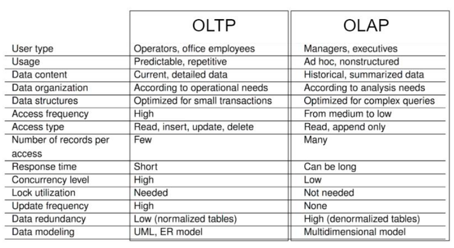
OLTP Systems → Operative databases (elaboration of online transactions) OLTP are traditional databases optimized to support daily operations:
-
Rapid access to data
-
Elaborating transaction
-
Comparison given updated coherent online data Proprieties of OLTP
-
Detailed data
-
No historical data
-
Highly normalized
-
Bad performances on complex queries
Data analysis requires a new paradigm, OLAP
-
Focuses on analytic queries, where data reconstructions
-
Support for loads of heavy queries
-
Indexing aimed to access few records
-
OLAP queries include aggregation
at DW backend we have
-
ETL tools
-
Data staging → intermediate database where all the modification processes get executed at DW level we have
-
Enterprise DW → centralized warehouse, includes organization
-
Data mart → DW of specialized departments
-
Metadata →
- Enterprise metadata → describe semantics and rules, constraints and politics of data. Security and monitor info. They describe data sources (schemes, proprieties, update frequencies, limits, access methods)
- Technical metadata → describe data storing and apps and processing acting on data ( ETL operations ). They describe the structure of DW and Data mart, at a conceptual/logical level, and physical level
- Repository → memorizes info on DW and its contents at OLAP level we have → a server that provides a multidimensional view of data a Frontend has
-
visualization of data
-
client tools to use the contents of the DW
-
OLAP tools → provide interactive exploration and manipulation of data, and the formulation of complex queries ad hoc
-
Reporting tools → reports management and production, they use predefined queries used regularly
-
Static tools → analysis and visualization of data cubes trough static methods
-
Data mining tools → allow users to analyze data to acquire knowledge on models and tendencies, used to make predictions
Multidimensional model (MultiDim) MultiDim visualizes data in a -dimensional space, a cube composed by dimensions (perspectives of data analysis) and facts
-
-
Example Dimensions → Client, Time, Product. Dimensions are described by attributes. Facts → Sales. every cell of the cube is the no. of units sold per category, time unit and a client’s city Measures → Quantities
-
Additive → summary trough addition (the most common one)
-
Semi-additive → summary trough addition of some dimensions (not all)
-
Non-additive
-
Distributive → defined by an aggregation function that can be calculated in a distributive way
-
Algebraic → defined by an aggregation function that can be expressed as a scalar function way
-
Holistic → cannot be calculated by under aggregated data. Members → instances of a dimension each cube of data contains different measures, a cube can be sparse or dense (since not all data could be present, eg. when there’s no data at all)
Data granularity → level of detail of measurements for each cube dimension (eg. Time: All - Year - Semester)
Hierarchies → can visualize data at different granularity levels. we can define mappings for the granularity levels, as well as a schema of a dimension
-
-
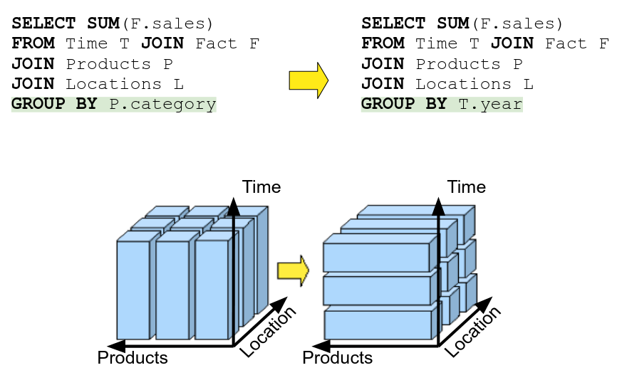
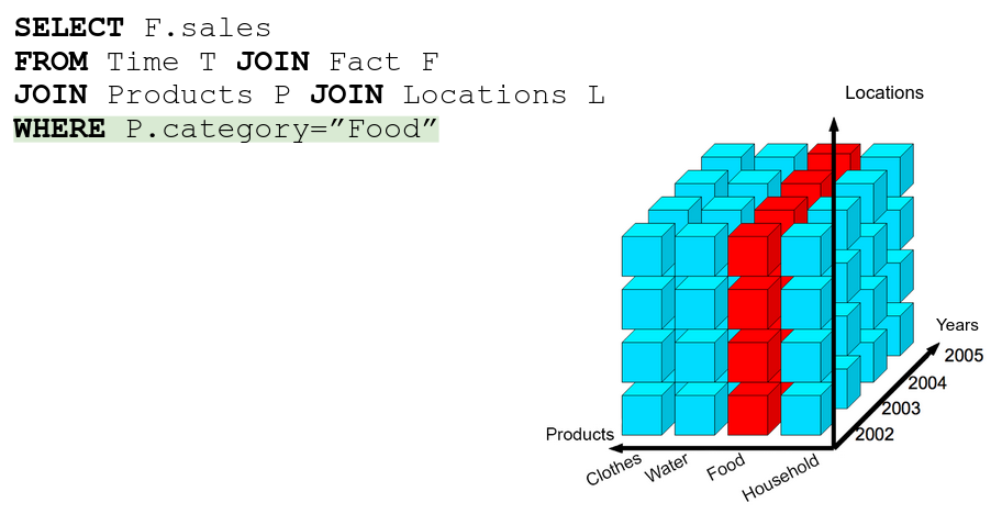
OLAP Queries for cubes (kinda useless) Roll-up → going to a higher level (specific to general) Drill-down → going to more specific levels (general to specific) In SQL, you access levels like so:
SELECT SUM(F.vendite)
FROM Time T JOIN Fatto F
GROUP BY T.year <----
WHERE T.year = 2018
Pivot → rotation of the cube, basically changing the group by
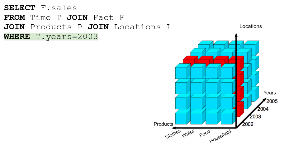
 Slice → just a WHERE statement
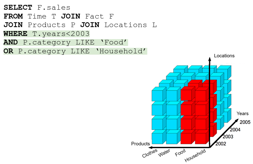
 Dice → selecting more than 1 slice, literally an AND/OR in the WHERE
4.3 Data Mining
Data mining → computing process of discovering patterns in large data sets involving methods at the intersection of machine learning, statistics and db systems
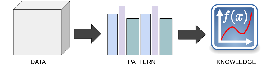 Patterns → regularities, patterns (eg. house prices are roughly 2500€ per , buying cereals and buying milk)
Knowledge → understanding the logic behind the patterns. to get knowledge we need big data and different observations on homogeneous data
Patterns → regularities, patterns (eg. house prices are roughly 2500€ per , buying cereals and buying milk)
Knowledge → understanding the logic behind the patterns. to get knowledge we need big data and different observations on homogeneous data
-
Data extraction steps
-
Problem definition
-
Identify required data
-
Pre-elaboration → clean the data so that can be input to a ML algorythm
-
Hypothesis modulation
-
Training and testing
-
Verify and distribute
Machine Learning
-
-
Does the abstraction from data to patterns.
-
Non linear interactions are hard to spot
-
Manual codification of some algorithms can be hard
-
(almost) never 100% accurate Supervised techniques → we use a “training set” of data with a variable that is the “solution”, acting as output examples
Supervised learning has to
-
Regression (if output is a numerical value) → easy to calculate accuracy or error
-
Classification (if output is a class) →
- Binary classification (cat / not cat)
- Multi class classification → classes are a finite set of outputs
- Binary classification (cat / not cat)
-
Clustering → divides examples in clusters, similar examples in same cluster
-
Association rules → variable relations (eg. {onion, potato} → {hamburger})
-
Spotting anomalies → sus data gets sussed out
-
Generative models → from examples they generate an instance with similar characteristics
-
Characteristics extraction → reduces variables by generating new characterstics
Data pre-treatment A pre-treatment is common since real world data is incomplete, noisy and incoherent Pre-elaboration phases
-
Cleaning
- Deduction of missing data
- Identify wrong data, level noise data
- Correlate incoherent data
- Solve redundancy
-
Integration
-
Transformation
Denoising data Binning → populating bins of similar data and leveling each bin locally (averaging out values for each bin so they’re the same) Linear regression → searching the best line that can adapt attributes to favor previsions.
 Clustering → similar values are grouped together, values outside of clusters are anomalies and get scrapped.
Data Warehousing → uploading phase Data mining → machine learning phase
Data integration → combines entities and attributes from different sources
Entity identification table A and B
A.customer_id←>B.customer_numberhow do be disambiguate for sure?attribute metadata:
-
Attribute name → string distance between names
-
Attribute type → both string type
-
Value interval → both have the same interval of values impossible to be 100% accurate
Data transformation → data into vectors
Recall → hypothesis function modeled by AI
Codification problem → not all data is numerical
Scale problem → big numbers are not good in ML, since they work well on normalized values
Text codification to solve the codification problem, we just code the strings into vectors (Vectorization)
Bag-Of-Words (BOW) → every variable of a vector is a specific word with boolean values,
trueif the word appears in the text.Category codification Hot codification → same as BOW, but every variable is a category, and only 1 can be true
Resizing (Normalization) → better performance and precision in ML, usually obtained trough linear resizing.