CV Insights and Summaries

Insights

---

The profs uses all range of the voting (from 18 throughout 30) when making students pass, unlike other prof tendencies of using 26-28-30 in magistrale. He’s exigent but doesn’t push you during the oral exam, giving you time to explain and thinking about the question. The theory is a lot of stuff for 6 CFU if that wasn’t obvious enough. As far as i know the presentation can be done in english or italian alike. The prof can ask some questions during the presentation of the project, and since 99% of projects and papers are about machine learning, after the presentation the theory question will travel towards the general part (part 1 in my notes). This means you could selectively study the 2nd part from everything around your project in depth theory-wise and then focus on the 1st part of the course, a little easier imo. Your call, i already studied everything anyway and i’m prepared for whatever will come my way.

Summaries

---

Part 1, Classic vision

---

Computer vision → field for information extraction from images

1. Image Formation Process

From 3D scene to 2D image, we need to

• Geometric relationships, 3D point in 2D pic
• Radiometric relationships, light info
• Digitization

Pinhole model → tiny hole that captures light rays We convert 3D points in a 2D image plane following the rules of perspective projection

Stereo model

Stereo model → using 2 images to recover 3D structure by triangulation (2 point distance difference, the higher, the further the points are in depth)

$\text{depth }z=\frac{\text{baseline }b\cdot \text{focal length }f}{\text{disparity }d}$ Epipole → point in one stereo image that lines with the point where the 1st photo was taken E Epipolar line → corresponding points lie on the same epipolar lines in both images

Digitalization

Sensors convert light to electrical signals Key processes:

• Sampling → space, colour discretization in pixels, hue
• Quantization → light discretization in brightness

Sensor characteristics

• Signal-to-noise ratio, measures noise in signals
• Dynamic range → range of detectable light levels Colour sensor → optical filters placed in front of photo detectors, capture specific colour channels (R,G,B)

2. Spacial Filtering

reduce noise (Denoising) in images using pixel neighbours info

• Mean across time with multiple images
• Mean across space with neighbour pixels Image filters → compute a new RGB value for each pixel based on neighbour pixels (denoising, sharpening, edge detection)

Filter kernel → small matrix that “slides” trough the image, used for calculating the output

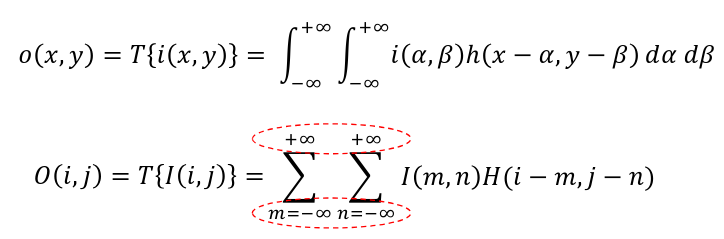
Linear and Translation-Equivariant (LTE) operators → filter type, used as feature extractors in CNNs (Convolutional Neural Networks) Implemented via 2D convolution between the image and a kernel (impulse response).

Translation-equivariant operator → If you shift the input, the output shifts the same way.

Convolution

properties

• Associative
• Commutative
• Distributive
• Convolution Commutes with Differentiation The properties make convolutions easily applicable in pipelines in any order

Correlation is the same as convolution without flipping the kernel

Discrete convolution

Border issue solved with

• Cropping the image
• Padding the image (duplicate/reflect)

Linear filters

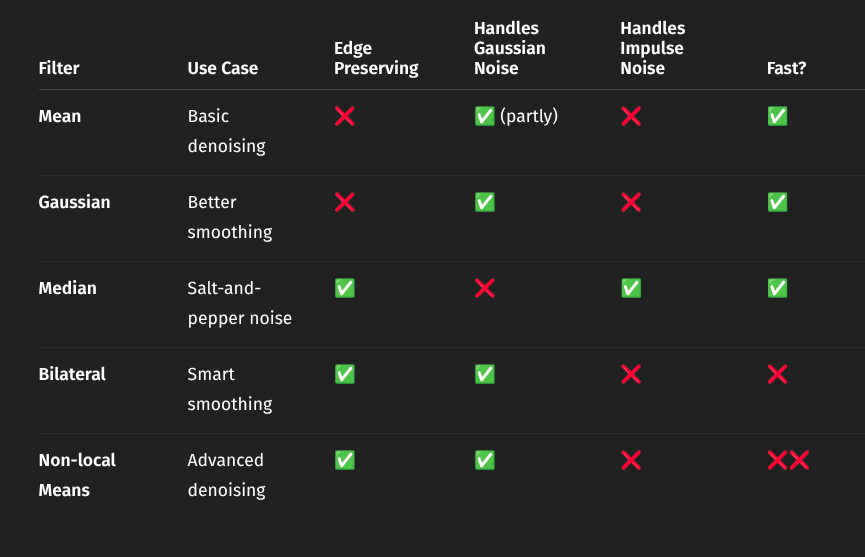
• Mean Filter → replace pixel intensity with the average intensity of neighbourhood, Fastest way to denoise an image
• Gaussian Filter → LTE operator whose impulse response is a 2D Gaussian function $\sigma$ standard deviation param → amount of smoothing by the filter (higher → more blur), defines the size of the kernel filter

Non-linear filters

• Median Filter → each pixel intensity is replaced by the median over a given neighbourhood, the median being the middle value in the sorted neighbourhood.
• Bilateral Filter → Advanced non-linear filter to accomplish denoising of Gaussian-like noise without creating the blurry effect on edges.
• Non-local Means Filter → non-linear edge preserving smoothing filter. Finds patches across the image that look similar and averages their center pixels

Summary/Characteristics

3. Edge Detection

Edges seen as sharp brightness changes

Brightness changes and therefore edges are detected with threshold over the 1st derivative

Gradient approximation

in 2D, we calculate the gradient (vector of partial derivatives) that detects direction of the edge

• Magnitude = strength of edge
• Direction = towards brighter side We approximate the gradient by estimating derivatives with
• Differences (pixel difference)
• Kernels (same principle, using correlation kernels)

Noise workarounds

Noise causes false positives, so we smooth the image when detecting edges

Prewitt/Sobel ops make so we take into consideration the surrounding pixels to evaluate the edge Prewitt operator → take 8 surrounding pixels Sobel operator → likewise but central pixels weight 2x

Non-Maxima Suppression (NMS)

strategy of finding the local maxima in the derivative

• We need to find the gradient magnitude from the approximation
• We use Lerp from the discrete grid’s closest points To get rid of noise we apply a threshold

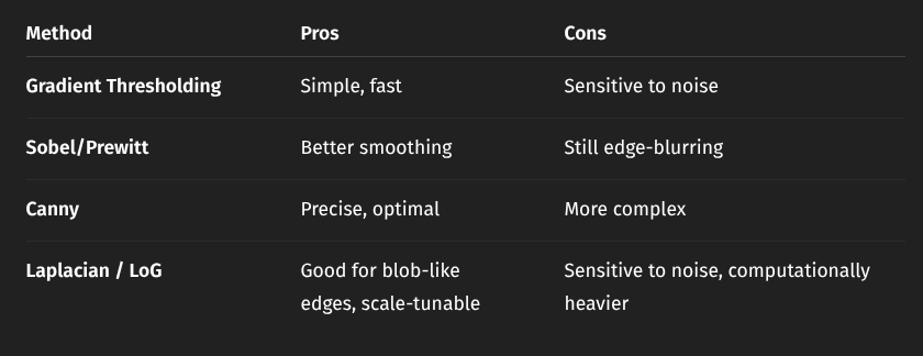
Canny’s Edge Detector

Standard criteria

1. Good detection → extract edges even in noisy images
2. Good localization → minimize found edge and true edge distance
3. One response to one edge → one single edge pixel detected at each true edge

Canny’s Pipeline

1. Gaussian smoothing
2. Gradient computation
3. Non-maxima suppression
4. Hysteresis thresholding → approach relying on a higher $(T_h)$ and a lower $(T_l)$threshold.

2nd derivative edge detection methods

Zero crossing = get point at 0 of 2nd derivative Laplacian operator (sum of second-order derivatives) to approx derivatives ${\nabla }^{2}I=\frac{{\partial }^{2}I}{\partial x^2}+\frac{{\partial }^{2}I}{\partial y^2}$

Laplacian of Gaussian (LOG)

Pipeline

1. Gaussian smoothing
2. Apply Laplacian
3. Find zero-crossings
4. Get actual edge from where the abs value of LOG is smaller

Parameter sigma controls smoothing degree and scale of features to detect (we blur more if edges are “bigger”)

Comparison

4. Local Features

find Corresponding Points (Local invariant features) between 2+ images of a scene

Three-Stage pipeline

1. Detection of salient points
   • Repeatable, find same keypoints in different views
   • Saliency, find keypoints surrounded by informative patterns
   • Speed
2. Description of said points (what makes them unique)
   • Distinctive - Robustness Trade-off, capture invariant info, disregard noise and img specific changes (light changes)
   • Compactness, low memory and fast matching
   • Speed
3. Matching descriptors between images

Corner detectors

corners are the perfect keypoints as they have changes in all directions

Moravec Interest Point Detector → Look at patches in the image and compute cornerness (8 neighboring patches, look for high variation)

Harris Corner Detector

1. Compute image gradients (how intensity changes)
2. Build the structure tensor matrix $M$
3. Compute the corner response $C=\det (M)-k\cdot \text{trace}(M{)}^2$
4. Threshold & NMS to pick the best corners

Harris invariance properties

• Rotation invariance
• Partial illumination invariance (if contrast does not change)
• No scale invariance

Scale-Space, LoG, DoG

Key finding → apply a fixed-size detection tool on increasingly down-sampled and smoothed versions of the input image (trough Laplacian of Gaussian or Difference of Gaussian, its approximation) (LoG, DoG)

Scale-space → group of the same image at different computed smoothed scales $L(x,y,\sigma )=G(x,y,\sigma )\ast I(x,y)$ Where:

• G is the Gaussian kernel
• $\sigma$ controls the scale (blur amount)
• $\ast$ is convolution

Multi-Scale Feature Detection (Lindeberg) → makes us find which feature to extract at what scale

• Use scale-normalized derivatives to detect features at their “natural” scale.
• Normalize the filter responses (multiply by $\sigma$)
• Search for extrema (maxima or minima) in x, y, and $\sigma$ i.e., in 3D with LoG.

LoG → second order derivative that detects blobs (circular structures) $F(x,y,\sigma )={\sigma }^2\cdot {\nabla }^{2}L(x,y,\sigma )$ DoG → approximation of LoG $DoG=L(x,y,k\sigma )-L(x,y,\sigma )$ We build a pyramid of images blurred with different $\sigma$ and we compute the difference to find the extrema in 3D across (x,y, scale)

• We reject low contrast responses
• We prune keypoints on edges using the hessian matrix We get the optimal scale for each detail

DoG invariance

• Scale invariance
• Rotation invariance (compute canonical orientation so that we have a new reference system different from the image’s)

SIFT Descriptor

Scale Invariant Feature Transform → used to generate descriptors to match, outputs a feature vector based on grid subregions (takes small details from around the keypoint and remembers gradient orientation combinations)

Matching process

find closest corresponding point efficiently, classic Nearest Neighbour problem

• distance used is the euclidean distance
• ratio test of distances to eliminate 90% of false matches (distance to best match/second best), small ratio = confident match Indexing techniques are exploited for efficient NN-search
• k-d tree
• Best Bin First

5. Camera Calibration

We need to measure 3D info accurately from the 2D img Camera calibration → determining a camera’s internal and external parameters (focal length, distortion / position, orientation).

Perspective projection

3D point $M=[x,y,z{]}^T$ projected into 2D image point $m=[u,v{]}^T$ Function:

$$\{\begin{array}{l}u=\frac{f}{z}x\\ v=\frac{f}{z}y\end{array}$$

where: $f$ → focal length $z$ → depth (distance from the camera) This projection is non-linear, aka objects appear smaller with distance, all the rules of perspective

Projective Space

we need to handle points at infinity Projective space ($P^3$) → 4th coordinate for each point in 3D, $[x,y,z,w]$ $w\in [0,1]$, 0 means point is at infinity Express perspective projection linearly using matrix multiplication: $\tilde{m}=P\cdot \tilde{M}$

• $\tilde{M}$: 3D point in homogeneous coordinates $[x,y,z,1]$
• $\tilde{m}$: projected 2D image point $[u,v,1]$
• $P$: Perspective Projection Matrix (PPM) Canonical PPM (assuming $f=1$) $P=\left[\begin{array}{cccc}1& 0& 0& 0\\ 0& 1& 0& 0\\ 0& 0& 1& 0\end{array}\right]$

Image Digitization

continuous measurements into discrete pixel size, img origin Steps

1. Scale by pixel dimensions $\Delta u,\Delta v$
2. Shift the image center to pixel coordinates $(u_0,v_0)$ Intrinsic Parameter Matrix $A$ → captures internal characteristics of the camera $A=\left[\begin{array}{ccc}{f}_x& s& u_0\\ 0& f_y& v_0\\ 0& 0& 1\end{array}\right]$ Where:

• $f_x=f\cdot k_u$ →: focal length in horizontal pixels
• $f_y=f\cdot k_v$ → focal length in vertical pixels
• $s$ → skew (typically 0 for most modern cameras)
• $(u_0,v_0)$ → image center

CRF = Rotation matrix $\cdot$ WRF + Translation vector

Homography $H$

flat scene whose projection we can simplify to an homography $\tilde{m}=H\cdot \tilde{M}$ Where:

• $H$ → 3x3 matrix representing the homography
• $\tilde{M}$ → 2D coordinates in the plane + 1 in homogeneous coordinates (quadruple) Simplifies calibration, holds info about intrinsic parameters

Lens distortion

Barrel → outward bending Pincushion → inward bending we need to model non-linear functions to correct the image

What is calibration

Calibration estimates:

• Intrinsic parameters $A$ → Capture multiple images of a known pattern (e.g., chessboard)
• Extrinsic parameters $R,T$ → Find 2D-3D correspondences (image corner ↔ real-world corner)
• Lens distortion coefficients → projection equations

Zhang’s method

A Practical way to calibrate a real camera using images of a flat pattern

1. use a flat target (all $z=0$ )
2. form $m\leftrightarrow M$ pairs, get homographies $H_i$
3. Each homography relates image coordinates to pattern coordinates 4.5 points per image needed to compute $H_i$

Summary

Concept	What It Represents
$A$	Intrinsic matrix (focal lengths, image center, skew)
$R,T$	Camera pose (extrinsics)
Homography $H$	2D projective mapping for planar scenes
Distortion	Lens imperfections modeled with parameters
Zhang’s Method	Practical way to calibrate a real camera using images of a flat pattern

Part 2, Modern vision

---

6. CNN recap (Convolutional Neural Networks)

Representation learning → do the tasks described in classic vision with deep learning

CNN Components

• Input image → passes through layers → abstract features are learned

1. Convolutional layers
   • extract features (patterns) from input, slides kernels across
   • creates feature maps
2. Activation functions
   • learn more complex patterns but introduces non-linearity (ReLU function, negative values to 0)
3. Pooling layers
   • reduce spatial size of feature maps (max pooling, avg pooling)
4. Fully connected layers
   • neuron connected to prev, helps with decision making
   • makes classification/regression happen
5. Loss functions
   • measure “correctness” and tries to improve the network
   • Cross-entropy, mean squared error are loss functions
6. Optimizers
   • Changes network’s weights to minimize loss functions
7. Normalization
   • Standardizes layer outputs, stability of network
8. Regularization
   • prevents overfitting
   • helps the model to generalize

Gradient descent optimizer

Gradient descend → how the model learns, tells the model “which way” to minimize the loss function

Steps:

1. compute the loss $J$
2. Calculate the gradients (derivatives of the loss with respect to each parameter)
3. update parameters using the following formula 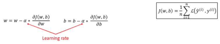Where:

• $\alpha$ → learning rate
• $w,b$ → weights, biases
• $\frac{\partial J}{\partial w},\frac{\partial J}{\partial b}$​ → gradient of the loss Repeat process while keeping on minimizing loss (“learning”).

loss functions are full of local minima, saddle points, flat regions

Stochastic Gradient Descent → approx of gradient descent, use mini-batches (small random portions of whole dataset)

• Introduces noise that prevents overfitting
• One epoch → whole training set observed one time
• Batch size → how many samples per update

Optimizers

1. Momentum
   • moving average of past gradients, move in that direction
2. RMSprop Root Mean Square Propagation
   • moving average of squared gradients
3. Adam Adaptive moments
   • combination of Momentum and RMSprop

Hyperparameters → every optimizer has them, stuff like learning rate, decay rates

Convolutional layers

Basics Images → 3D tensors (height, width, channels) Filters (kernels) → slide over the image and extract patterns Outputs an activation map (feature map)

Filter depth = image depth

Padding → convolution operator shrinks the output, we add padding to the image to preserve size Stride → movement of the filter, stride 1 = slide 1 pixel

Deep CNNs, Pooling, Receptive fields

Deep CNNs are made by stacking

1. Convolution + ReLU
2. Pooling (max) Called feature extractor

Pooling → Reduces resolution, keeps dominant features.

• Max pooling (most common): picks the max value in a patch.
• Average pooling: averages values (less common in modern CNNs).

Receptive field of a neuron → neuron’s POV in an image deep layers = bigger receptive fields

Batch normalization

network stabilization to avoid gradient vanish/explode BatchNorm normalizes layer outputs and it’s the standard in modern CNNs Given:

• A mini-batch of activations $\{z^{(1)},\dots ,z^{(m)}\}$
• $m$ → batch size We do

1. Compute the batch mean $\mu$
2. Compute the batch variance $\sigma$:
3. Normalize each activation
4. Scale and shift (learnable parameters)

Regularization

preventing overfitting, 3 methods

• Dropout → During training, randomly remove (“drop”) some neurons so the network doesn’t rely on any one path too much.
• Early Stopping → Stop training before the model starts to overfit.
• Cutout (a kind of data dropout) → Mask out parts of the image at random to force the model to look beyond obvious features.

Data augmentation

artificially increasing your training dataset from existing imgs

• flip, rotate, resize, color jitter → same object under difference transformations
• cutout → learn less obvious features
• multi-scale training → different sizes flexibility

7. Object Detection

A detection provides:

• A category label (eg “car”, “dog”)
• A bounding box

Viola-Jones Detecting faces

Haar-like features → Simple rectangular contrast patterns, 24x24 patches of the image Those are optimized with

• Integral images → pre-processing pixel sums for rectangles computation
• AdaBoost algorithm → weak learners into a strong classifier
• Cascade → early rejection

Sliding window + CNN, Naive extension

use CNN as a sliding window detector, predict class and bounding box for each window Non-Maximum Suppression (NMS) Algorithm → pick the highest-scoring detection and discard all significant boxes overlap (Intersection over Union > threshold) too many windows, slow and expensive

Region proposals (R-CNN Series)

estimate regions to check and apply deep learning there

R-CNN (Region-CNN) → selective search to generate candidate object regions, using low level features Fast R-CNN → run CNN once over image, get feature map and use Rol Pooling to extract region features, Predict trough fully connected layers class scores and bbox corrections Faster R-CNN → Introduces the Region Proposal Network (RPN)

• We give in input boxes anchors for each region that the RPN uses to compute objectness score
• Positive samples: anchors with IoU ≥ 0.7 with a ground truth box
• Negative samples: anchors with IoU < 0.3 with all ground truth boxes we use positive samples to get the mini-batch we use for training

One-Stage Detectors

small accuracy, very fast and simple

1. YOLO
   • SxS grid, backbone CNN gets the feature map
   • for each grid cell in feature map, get presence, bounding box and class % directly into the grid
2. SSD
   • Backbone extracts feature maps from detectors at multiple scales
   • extra feature layers are added
   • use anchors
   • can predict multiple objects in the same location
3. RetinaNet
   • FPN (Feature Pyramid Network) → creates “pyramids” of high-res features at every level of resolution, helps with different sizes of objects
   • Tackles class imbalance with Focal Loss using a focus parameter, making the model learn on hard examples

Anchor-Free Detectors – CenterNet

Anchors have downsides in the form of

• manual design for ratios,
• heuristics,
• need for NMS to avoid duplicates,
• inefficient and non-differentiable post-processing.

Use central points of objects

• Output heatmap, 1 channel per class, brightens center of object
• Offset map corrects stride errors (discretization)
• Size map predicts $w,h$ bbox on centered object, found by local maxima on heatmap

Summary

Generation	Approach	Key Features	Trade-off
Viola-Jones	Hand-crafted features	Fast, real-time face detection	Only for specific objects
R-CNN series	Two-stage, region-based	High accuracy, flexible	Slower
YOLO/SSD	One-stage, grid-based	Real-time, simple	Lower accuracy
RetinaNet	Focal loss for imbalance	One-stage with improved accuracy	Still uses anchors
CenterNet	Anchor-free, point-based	Simpler, end-to-end	Still evolving in accuracy

8. Segmentation

classify every pixel with a category label

Evaluation Metrics

• IoU (Intersection over Union) → How well do the predicted and real masks overlap?

• mIoU (mean IoU) → Average IoU across all classes. (most balanced, widely used)

• Pixel Accuracy → How many pixels were correctly labeled?

• Mean Accuracy → Per-class accuracy.

• Frequency-Weighted IoU → Gives more weight to common classes.

Segmentation masks prediction

Fully Convolutional Networks → CNNs where we have only convolutional layers, so we have spatial maps instead of labels

We upsample the output with Interpolation (simple) or Transposed convolutions (learned) We keep details by “skip connection” from earlier layers to retain the detail to sum/concat into the output

Transposed convolutions - Learnable upsampling

convolutions reduce size, transposed convolutions go the other way

We use the kernel to expand the input value, contribution summed on overlap. Works like a conventional operator (eg. bilinear interpolation), but the Kernel is tailor made by AI.

U-Net → Encoder–Decoder for Segmentation

U-Net → specialized architecture for segmentation:

• Encoder: Compresses the image (like any CNN).
• Decoder: Reconstructs the mask.
• Skip connections: Combine encoder and decoder features.

Dilated Convolutions (Atrous Convolutions)

insert gaps between kernel elements, making them “see” larger regions of images. $r$ → dilation rate parameter Dilated convolutions let us retain spatial resolution while still seeing a large part of the image. “zoom out” effect, possible to lose fine features

Instance Segmentation = Detection + Segmentation

difference instances of objects Mask R-CNN → Extension of Faster R-CNN

• Adds a segmentation head
• Predicts a binary mask per region. This mask:
  • Has a fixed resolution (e.g., 28×28),
  • Is specific to one object proposal.

Rol-Align → rol pooling improvements by exploiting misalignments with bbox and segmentation:

• Not rounding coordinates → uses exact floating-point positions.
• Bilinear interpolation → samples feature map values precisely.
• Pooling values more smoothly (via max or average). Once the RoI features are extracted:
• They are fed into a small Fully Convolutional Network (FCN).
• This FCN outputs a mask per class, typically sized 28×28.

Modular design, expandable (eg. Keypoint detection)

Panoptic segmentation = The Sky and a Person

everything we segment has an ID Implementation: Panoptic Feature Pyramid Networks (FPN) Based on Mask R-CNN, this model:

1. Uses FPN features for both semantic and instance heads.
2. Adds a segmentation branch for stuff categories.
3. Merges outputs, resolving overlaps and inconsistencies.

9. Metric Learning

Embedding learning → no classes, structured space where intra-class distances are minimized

Siamese Networks and Loss Functions

Siamese networks → two+ identical networks with shared weights, trained on pairs of inputs, they train based on similarity

k-Nearest Neighbors (k-NN)→ Algorithm used for classification and regression. When given a new data point, k-NN looks at the k closest data points (neighbors) from the training set based on a distance metric like Euclidean distance and decides.

Contrastive loss → minimize distance between same class imgs, penalize close different classes, include a margin to prevent over-pushing dissimilar pairs

Triple Loss

Triplet Loss → (Positive, Anchor, Negative) triplet ensures closeness of positive to anchor in relation to the negative distance more direct than contrastive loss, can collapse.

semi-hard negatives optimization → examples that are between the positives and the margin so they contribute non-zero loss

Applications

• Img retrival
• Re-identification
• Few-shot learning
• E-commerce (item recognition)

10. Transformers

same as word2vec base idea

Recurrent Neural Network (RNN)

network that processes sequential data using a hidden state that “remembers” previous inputs $h(t)$ → hidden state at step $t$, same set of weights used every step, generalizes with different sequence of lengths

RNN is a “loop”, unrolling in training so we can apply backpropagation trough time

We compute loss at each step, summing each step for the current and total loss.

it’s hard to learn long-range dependencies because of vanishing (mostly) or exploding gradients…

Encoder-Decoder architectures

• An Encoder processes the input sequence. The encoder emits the context $C$, as a function/vector of its final hidden state
• A Decoder takes that context $C$ and generates the output sequence in a sequential way Bottleneck = encoder output (single vector)

Solution: focus on specific parts of the context vector, Attention mechanism → make the decoder assign weights (trough attention scores) to all encoder states, so it knows where to focus for each output word

Transformers

Uses only self-attention (and cross-attention), removes RNNs sequentiality

• At each step the model is auto-regressive, consuming the previously generated symbols as additional input when generating the next
• Input-outputs are the same as encoders-decoders in RNNs

Transformer Encoder

1. get the dense vector of each word (token), vector size d_model
2. Add positional encodings to give a sense of order (vector of size d_model)

having N layers made by

1. Multi-Head Self-Attention
2. Feed-Forward Neural Network (FFN) Each of these sub-layers has:

• Residual connections (skip connections)
• Layer Normalization (all vectors of size d_model) → stabilizes the model in train

Transformer Decoder in CV, decoders are made ad-hoc so we don’t care about them

Self Attention

How the model understands context: we look at each token focusing on other relevant tokens in the same sequence.

How to calculate attention:

1. from the input vector in the encoder, we multiply it by 3 weight matrices learned during training, resulting in
   • Query (Q): What this token is looking for.
   • Key (K): What each other token has to offer.
   • Value (V): What information each token carries.
2. Get how similar every Key is with the Query with Similarity
3. Use Softmax on similarities to get attention scores
4. Use scores to compute a weighted sum of all Value vectors

Multi-Head Attention → self-attention multiple times with different weights to understand different aspects we’re looking for

Vision Transformers (ViT)

Encoder for images

1. We split images into fixed size patches (DINOv2 is 14x14)
2. Patches are our tokens
3. We add positional encodings to retain spatial information
4. Feed the patch sequence into a standard Transformer encoder. We adapt the input to treat it so it was a sentence