Conceptual maps

🐰 i cannot fathom to remember anything about theory, i can’t explain theoretical concepts no matter how much i try to understand them, they slip my mind. I’ll try making conceptual maps to train me more to remember

1. Image Formation Process

Getting a 3D scene into a 2D image

1. Geometric information
   1. Perspective projection
   2. Stereo vision
2. Digitization
   1. Sensors for sampling (space/colour) and quantization (light)

2. Spacial Filtering

Reduce noise in images

1. Concept of denoising
2. Filters, compute new RGB value for each pixel
3. Linear and Translation-Equivariant type of filter
4. Convolution properties
5. Discrete convolution → sum product of the 2 signals with 1 being reflected
6. Filters
   1. Linear
      1. Mean filter
      2. Gaussian filter → further pixels are less important
   2. Non-Linear
      1. Median filter → middle value
      2. Bilateral filter → further or different pixels are less important
      3. Non-local Means filter → find similar patches

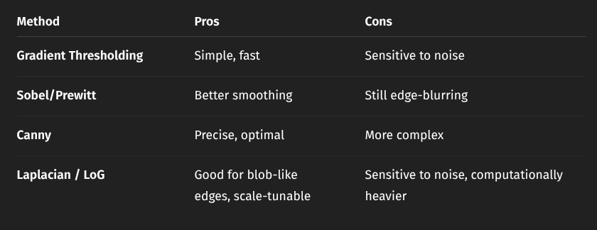
3. Edge Detection

1. 1D step edge → 1st derivative
2. 2D Gradient → compute partial derivatives to get direction and strength
3. Discrete approximation → differences in pixels
4. Noise
   1. Prewitt and Sobel operators → decide weights of current pixel based on brightness difference of surroundings
5. Non-Maxima Suppression (NMS)
   • Find local maxima along gradient
   • Estimate direction locally (with Lerp from closest pixels)
   • Thresholds
6. Canny’s criteria
   1. Good detection
   2. Good localization
   3. One response, one edge
7. Canny’s edge detector PIPELINE
   1. Gaussian smoothing
   2. Gradient computation
   3. Non-maxima suppression
   4. Hysteresis thresholding
8. 2nd order derivative methods
   1. zero crossing
   2. Laplacian operator (sum of 2nd order derivatives) approximation
9. Laplacian of Gaussian (LoG) PIPELINE
   1. Gaussian smoothing
   2. Apply Laplacian operator
   3. Find zero-crossings
   4. localize edge at sign change
10. Summary
    • 

4. Local Features

find Local invariant features (corresponding points) in images

1. Three-stage pipeline
   1. Detection
   2. Description
   3. Matching
2. Properties
   • Detector
     • Repeatability
     • Saliency
   • Descriptor
     • Distinctiveness vs. Robustness Trade-off → get invariant info
     • Compactness
   • Desirable speed for both
3. Corner detectors
   1. Moravec detector → look at patches and compute cornerness (high variation)
   2. Harris corner detector
      1. Compute gradients around point of interest, create matrix with results
      2. Compute corner score with matrix
      3. Threshold & NMS to pick the best corners
   3. Invariance properties of harry’s detector
      1. Rotation invariance
      2. Partial illumination invariance (only uniform shift)
4. Scale space → concept of same img at different scales
5. Linderberg (multi-scale detection)
   1. Use scale normalized derivatives
   2. Normalize filter responses
   3. Search extrema in 3D
6. Scale-normalized LoG → filter (second order derivative) that detects blobs (circular structures)
7. Difference of Gaussian (DoG) → approx of Scale-normalized LoG, find extrema across results in 3F
8. Invariance of DoG
   1. Scale invariance
   2. Rotation invariance (get canonical orientation, remember local coords)
9. SIFT Descriptor → Scale invariant feature transform
   1. take 16x16 grid around keypoint
   2. 4x4 subregion division
   3. 8-bin histogram if gradient orientations
   • output vector is compact and robust
10. Matching process
    1. Nearest neighbour search, doing it efficiently
       1. k-d tree
       2. Best Bin First

5. Camera Calibration

determining a camera’s internal/external parameters to measure 3D info from 2D images

1. Perspective projection
   • WRF to CRF with Focal length and depth calculations
   • 4th coordinate for linear perspective projection
2. Digitization
   1. Intrinsic parameter matrix A, focal length xy, skew, central points
   2. Rotation matrix, Translation vector → relation CRF = R cdot WRF + T
3. Homography
   1. simplified projection
   2. taken from a flat image, depth 0
   3. Get planar targets, estimate matrix A
4. Lens distortion, Barrel / Pincushion
5. Calibration estimates:
   • Intrinsic parameters $A$
   • Extrinsic parameters $R,T$
   • Lens distortion coefficients
6. Zhang’s method → computes homography
7. Main Pipeline (Zhang’s method):
   1. Acquire images of flat pattern
   2. Estimate homographies $H_i$
   3. Use $H_i$​ to compute intrinsic matrix $A$
   4. Use $A$ and $H_i$​ to compute $R_i,T_i$ for each image
   5. Estimate lens distortion coefficients
   6. Use non-linear optimization to refine all parameters by minimizing reprojection error

6. CNNs

1. CNN
   • input image
   • layers
   • feature map output
2. Gradient descent → how the model learns
3. Optimizers
   1. Momentum
   2. RMSprop
   3. Adam (momentum + RMSprop)
4. Convolutional layers
   1. Padding to keep output size
   2. Stride
5. Deep CNNs
   1. Convolution + ReLU + Pooling
6. Batch normalization
   1. Avoid vanish/explode gradients
   2. compute mini-batch mean and variance, adjust learnable parameters by normalization
7. Regularization - prevent overfitting
   1. Dropout
   2. Early stopping
   3. Cutout
8. Data augmentation
   1. modify dataset to expand it
   2. flip, rotate, resize, jitter
   3. cutout
   4. multi-scale training
9. ResNet

7. Object Detection

Faster R-CNN → introduce Region Proposal Network, use anchors and samples

8. Segmentation

Classify area of objects 9. Evaluation metrix 1. Intersection over union 10. Segmentation masks predictions → uses fully convolutional networks for spatial maps 11. Transposed convolutions (upsampling) 12. U-Net → specialized encoder-decoder for segmentation, implements skip connections 13. Dilated convolutions - dilatate kernel to observe larger region, lose finer details - DeepLab - backbone CNN like ResNet - Remove strides and add dilation in later layers 14. Insance segmentation → classify different instances of class - Mask R-CNN, based on Faster R-CNN - Rol-Align - Bilinear interpolation for coords 15. Panoptic segmentation → get instances and general labels